Recession Ensemble
Ensemble probability
Model comparison
Why an ensemble
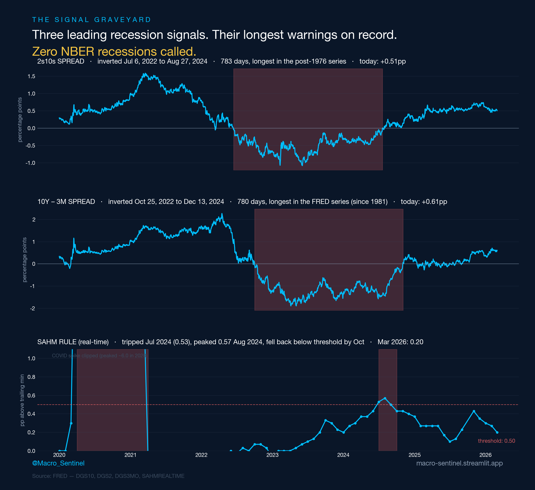
The two signals the ensemble leans on most — the yield curve and the Sahm rule — both gave their longest false-positive warnings on record this cycle. The 2s10s spread inverted for 783 days, the longest stretch in the post-1976 series. The 10Y–3M spread inverted for 780 days, the longest in the FRED series. The Sahm rule tripped at 0.53 in July 2024, peaked at 0.57 in August, and fell back below the 0.5 threshold by October — a textbook false fire.
NBER called none of it.
This is the case for an ensemble rather than any single signal. The multi-indicator logit (35% weight) reads broader stress — credit spreads, financial conditions, employment dynamics — and refused to confirm the curve and Sahm warnings when those broader channels stayed quiet. The classic signals are still load-bearing: 65% of the ensemble's weight sits on yield-curve probit and Sahm sigmoid combined. But they are checked against the rest of the macro-financial state, and the lesson of 2022–2024 is precisely why.
Methodology
Three models, three mechanisms, one ensemble. Each of the three component models captures a different recession mechanism; weights reflect the published and historical hit rates.
1. Yield-curve probit (40%)
Classic Estrella-Mishkin. A probit regression of the 12-month-forward NBER-recession indicator on the T10Y3M spread: $P(R_{t+12} = 1) = \Phi(\alpha + \beta \cdot (\text{10Y} - \text{3M}))$. Trained on the full available NBER-dated history. The yield curve's lead is long and consistent — this is the cleanest signal-over-noise model in the ensemble, and its 40% weight reflects that.
2. Multi-indicator logit (35%)
A logistic regression on a 7-feature panel (T10Y3M, T10Y2Y, HY OAS, BAA-10Y credit spread, NFCI, WEI, 3-month change in unemployment) plus the BCI common factor itself, walk-forward standardized. This model picks up non-yield-curve stress — credit spreads blowing out, employment turning, financial conditions tightening — that the pure curve model misses. Contemporaneous rather than forward-looking.
3. Sahm-rule sigmoid (25%)
The Sahm rule — 3-month average of U-3 unemployment minus the trailing-12-month low — becomes a proxy for recession as it crosses 0.5 percentage points. Here the raw reading is passed through a sigmoid mapping to $[0, 1]$. Sahm is a coincident signal, close to contemporaneous with recession onset — it's the ensemble's anchor against the two forward-looking models running hot when the economy is actually fine.
Ensemble
$P_{\text{ensemble}}(t) = 0.40 \cdot P_{\text{yc}}(t) + 0.35 \cdot P_{\text{mi}}(t) + 0.25 \cdot P_{\text{sahm}}(t)$
Static weights, no retraining. The risk-band thresholds (15 / 30 / 50 / 70) are published with the index and map the continuous probability onto an action-oriented label.
Canon
Estrella & Mishkin (1998, RES) — yield-curve probit methodology; Rudebusch & Williams (2009, JBES) — multi-indicator logit with financial-conditions features; Sahm (2019, Hamilton Project) — real-time Sahm rule for recession identification; Chauvet & Piger (2008, JBES) — dynamic-factor Markov-switching recession probabilities that inform the ensemble framing.
Inflation regime context
The recession ensemble's hit rate is influenced by the inflation regime — yield-curve inversions resolve to recession differently when CPI is running above 4% than when it's at target. The companion Inflation Nowcast page provides the forward 3m and 6m CPI nowcast that contextualizes the recession read. When the inflation nowcast is decelerating and the recession ensemble is rising, the regime is "stagdisinflation" — historically a difficult cross-asset environment.
Forward macro complements
Two additional calibrated nowcasts read the cycle from leading indicators rather than the financial-stress channels the ensemble uses:
- Wage Growth Nowcast — forward 6m / 12m Atlanta Fed Wage Growth Tracker. The Sahm-rule term (25% weight) reads unemployment directly; wage growth is the price side of the same labor market. When wage growth is decelerating and the Sahm sigmoid is rising, the cycle-end signal is reinforced.
- Industrial Production Nowcast — forward 3m / 6m INDPRO YoY. The logit term includes WEI, but INDPRO YoY is the production-side hard data that confirms or denies the financial-conditions read. INDPRO turning negative mid-cycle has historically been a high-conviction confirming signal alongside curve inversion.
Every prediction these pages emit lives on the Calibration Ledger — backfilled with as-if-live history and live-appending fresh rows on each loader run, so the published track record is auditable down to the as-of date.